2D Implicit Curves

Before we go into what are 2D implicit curves, I’ll first talk about 3D curves.

3D curves are defined as multivariate functions, in this form:

$$z = f(x, y)$$

For example, one of such 3D functions is this one:

$$\begin{equation}z = f(x, y) = \left(x^2 + y^2\right)\left(y^2+x\left(x+\frac{1}{2}\right)\right) - 4 \cdot \frac{1}{2} x y^2\end{equation}$$

To plot it, we use the z value of the function at x, y as an elevation. This forms a surface, provided the function is differentiable:

Implicit curves are curves that are defined as the intersection between a 3d curve and the XY plane.

For example, if we add the XY plane to the above graph, we get this:

The implicit function defined by the 3D curve is the little petals that emerge from the intersection between the XY plane and the curve.

In other words (or images 😝):

To summarize, the set of all (x, y) pairs where the 3D curve’s z value is zero form the implicit curve.

Plotting Curves

Drawing things is a search problem. It’s about finding the correct places to put pixels. Plotting curves is no different: we have some functions that, given some values, produce a specific result we are interested in (usually 0).

To plot those curves, we then must find all the inputs that after going through the functions give the desired result.

Intersection Test

When we are talking about plotting, we are also not interested in finding all the exact solutions to the function that defines the curve (there are infinite of those for most curves!). That happens because pixels are not points. Pixels have area. When we say we want to plot a pixel that is in a given implicit curve, we are talking about a pixel that intersects the curve.

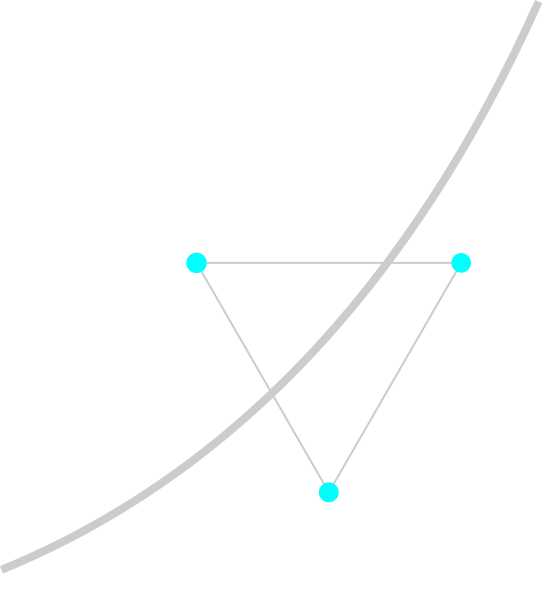
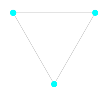
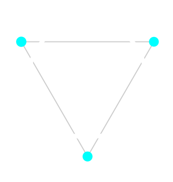
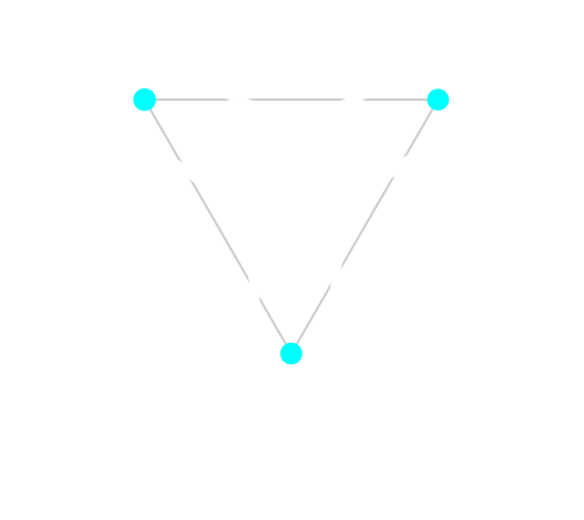
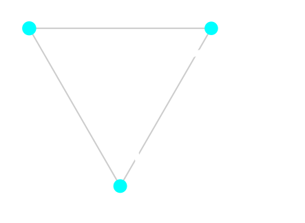
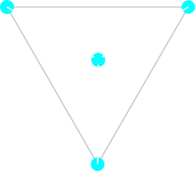
To check if a given small area contains part of the curve, we use the following test:

Given a triangle ABC, is this equality true? $$\frac{f(A)}{|f(A)|} = \frac{f(B)}{|f(B)|} = \frac{f(C)}{|f(C)|}$$ i.e.: does the function at all the points of the triangle have the same sign?

If all of them are the same sign, it means that the entire triangle is on the same side of the function. If they are not all the same sign, some of the points are on one side and the other are in a different side.

Because of the definition of a triangle itself, it is impossible to pass a line through it keeping all the points in a single side of the line, as illustrated below:

We can then use this test to know if the function passes through some are of the screen. In Rust we would write:

fn intersects_2_edges(f: Implicit, tri: Triangle) -> bool {
    (f(tri[0]).signum() +
     f(tri[1]).signum() +
     f(tri[2]).signum()).abs() as i32 != 3
}

Keep in mind this only works if the following conditions are held true:

1. the curve is differentiable
2. the triangle is very small (so the curve is nearly linear)

In cases where those two constraints are not respected, this simple algorithm may not detect the intersection with the function.

Triangle Subdivision

We now have a way of testing if some area of the screen contains part of the implicit curve. How can we expand that to actually plot the entire curve?

One way of doing that is first checking on which side of the screen the curve is (or if in both), then further dividing the sides that contain part of the curve and checking those, recursively. We do this until the size of the area is on the scale of a single pixel, then do a final test and paint that pixel if part of the curve is contained in the pixel.

This is not a new idea and is used in many algorithms. It’s essentially a form of binary search (or ternary, quaternary etc). The most famous example of a data structure using this is the quadtree algorithm.

We, however, want to subdivide triangles. Where exactly should we split a triangle to make sure the generated grid is uniform?

Thankfully, there’s a very simple algorithm for that:

We start out splitting the screen in two triangles. Then, for each triangle we put its points in an ordered tuple:

$$(A_1, A_2, A_3)$$

The order in which we put them is very important, because we always split from the A1 point into the midpoint of A2 and A3.

More precisely, each triangle (A1, A2, A3) can generate two new triangles given by:

$$ (A_1, A_2, A_3) \implies \cases{ (B_1, A_1, A_2) \cr (B_1, A_1, A_3) } $$

$$ B_1 = \frac{A_2+A_3}{2} $$

Notice that in the child triangles, B1 is the first point. As I said, the order is important because we always start splitting from the first point in the tuple. To keep the subdivision density even, the first point for the next subdivision should be the newly created (mid)point.

With this triangle subdivision algorithm and the triangle-curve intersection algorithm, we can then write a full plotting algorithm. In Rust:

fn tessellate_triangle(
    f: Implicit,
    tri: Triangle,
    depth: u32
) {
    if depth == MAX_DEPTH {
        // Draw pixel at tri's center
        return;
    }

    // Split the current triangle in two
    let children = [
        [(tri[1] + tri[2]) / 2.0, tri[0], tri[1]],
        [(tri[1] + tri[2]) / 2.0, tri[0], tri[2]],
    ];

    for child in children {
        if intersects_2_edges(f, child) {
            tessellate_triangle(f, child, depth + 1);
        }
    }
}

We start out from a triangle, subdivide it to form two new triangles. Then we check if the curve intersects the new triangles, if so continue the process recursively for them. Finally, once a given MAX_DEPTH has been reached, draw the pixel in the coordinates of the current triangle.

Efficacy of Subdivision-intersection

The algorithm above has one nice property: it’s simple. It only requires a few lines of code and understanding it is a matter of minutes. However, when it comes to actually plotting curves, it has a few issues.

All of those issues arise from the requirements we mentioned above for the intersection algorithm to work:

1. the curve is differentiable
2. the triangle is very small (so the curve is nearly linear)

Specifically, all of them come from not meeting the 2nd requirement. The 1st one should always be met from the definition of implicit curves.

Internal Curve

In this case all the points of the intersection test triangle have the same sign, but the function is contained inside it.

It could also have intersections and happen in the same way:

It’s still an internal curve in the sense that all points are on the positive side.

External Curve

In this case, even though parts of the curve are going inside the area of the triangle, all points in the triangle are still inside the curve (i.e.: on the negative side).

Single-intersection curve

This is a special case of an internal curve: all points in the triangle are on the positive side of the curve. However, it has its own section because it happens when the curve intersect only a single edge of the triangle. It can happen with nearly linear segments of the curve.

Improving Efficacy

Luckily, there’s one simple “trick” that can be used to improve the efficacy of this simple algorithm. Unfortunately, it takes away some of the beauty and speed and does not solve all the issues.

The core of this hack is to think back on why the issues happen: the curve is not linear enough to match the necessary conditions for the intersection algorithm to work properly. How could we make the curves more linear? The answer is: by subdividing more!

To subdivide more we define a minimum SEARCH_DEPTH to which we subdivide without making any tests. This will make the curve more linear in most cases. After that initial search phase we will have much smaller triangles, so we start actually checking intersections.

In Rust:

fn tessellate_triangle(
    f: Implicit,
    tri: Triangle,
    depth: u32
) {
    if depth == MAX_DEPTH {
        // Draw pixel at tri's center
        return;
    }

    // Split the current triangle in two
    let children = [
        [(tri[1] + tri[2]) / 2.0, tri[0], tri[1]],
        [(tri[1] + tri[2]) / 2.0, tri[0], tri[2]],
    ];

    for child in children {
        // +------- start by searching
        // |
        // v
        if depth <= SEARCH_DEPTH || intersects_2_edges(f, child) {
            tessellate_triangle(f, child, depth + 1);
        }
    }
}

This is actually a good enough algorithm depending on your application: you can tweak SEARCH_DEPTH and MAX_DEPTH to work well with most figures. The only issue is that for some of them you would require a very deep SEARCH_DEPTH, almost defeating the purpose of having this tessellation algorithm in the first place.

Tracing

So how can we improve this algorithm further? Turns out there’s a different algorithm altogether that we can combine with the subdivision-intersection! ☺️

The core of this new algorithm is that we find a single pixel that intersects with the curve. Then we search only the neighbor pixels to find which ones also intersect the curve, then repeat this recursively. Because we are working in the smallest unit of scale all the times (pixel), the curves are much more linear than with the subdivision algorithm.

If you raised an eyebrow 🤨 and thought “this looks like a flood fill algorithm”, you are right. This is a flood fill, the only difference is that the condition for filling is intersecting the curve.

Filling

We start from a point P1, then we check all its neighbor pixels. We fill the ones that intersect the curve and then start over from them, checking their neighbors.

One thing to note is that we need to keep track of visited pixels so we don’t run the algorithm again on them. We can do this using a grid, a hash map or some other data structure.

Translating to Rust:

pub fn trace(
    curve: Implicit,
    start: Point,
    filled: &mut HashSet<Pixel>,
) {
    let mut queue = VecDeque::new();

    // Some magic still going on here...
    match find_pixel_on_curve(curve, start) {
        Some(pixel) => queue.push_back(pixel),
        None => {}
    }

    while queue.len() > 0 {
        let pixel = queue.pop_front().unwrap();

        if !filled.contains(&pixel) {
            // Fill pixel

            filled.insert(pixel);
            queue.append(&mut VecDeque::from(find_neighbor_pixels(curve, pixel)));
        }
    }
}

You might have noticed that there’s still some ✨ magic ✨ going on here. How do we find the first point in the curve to start tracing?

Gradient

There’s an operation in calculus that we call the gradient of a multivariate scalar function.

The gradient is defined for each point the function is defined, as a vector pointing to the direction the function grows the fastest.

The way we know that is sampling how fast the function changes at that point for each of the variables and constructing a vector with those change speeds. If that sounds familiar, it is because this operation is just the partial derivatives of the function, and yes, the gradient is just a vector with all the partial derivatives at the given point.

Gradient is usually written with the symbol ∇, so, in mathy mathy:

$$ \nabla f(x, y) = \left[\begin{matrix}\frac{\partial f}{\partial x}(x, y)\cr\frac{\partial f}{\partial y}(x, y)\end{matrix}\right] $$

But how can this gradient be useful to us? It points in the direction the function grows. So if we take:

$$-\nabla f(x, y)$$

It should point us to the direction the function gets smaller, or in other words, to the direction zero is, which is what we want to find. There’s the caveat of negative numbers however, they get smaller as they get away from zero. To get around that we can use:

Given a point (x, y), the direction in which f goes to zero from that point is: $$-\nabla |f(x, y)|$$ or $$-\nabla f^2(x, y)$$ Provided that there are no local minima.

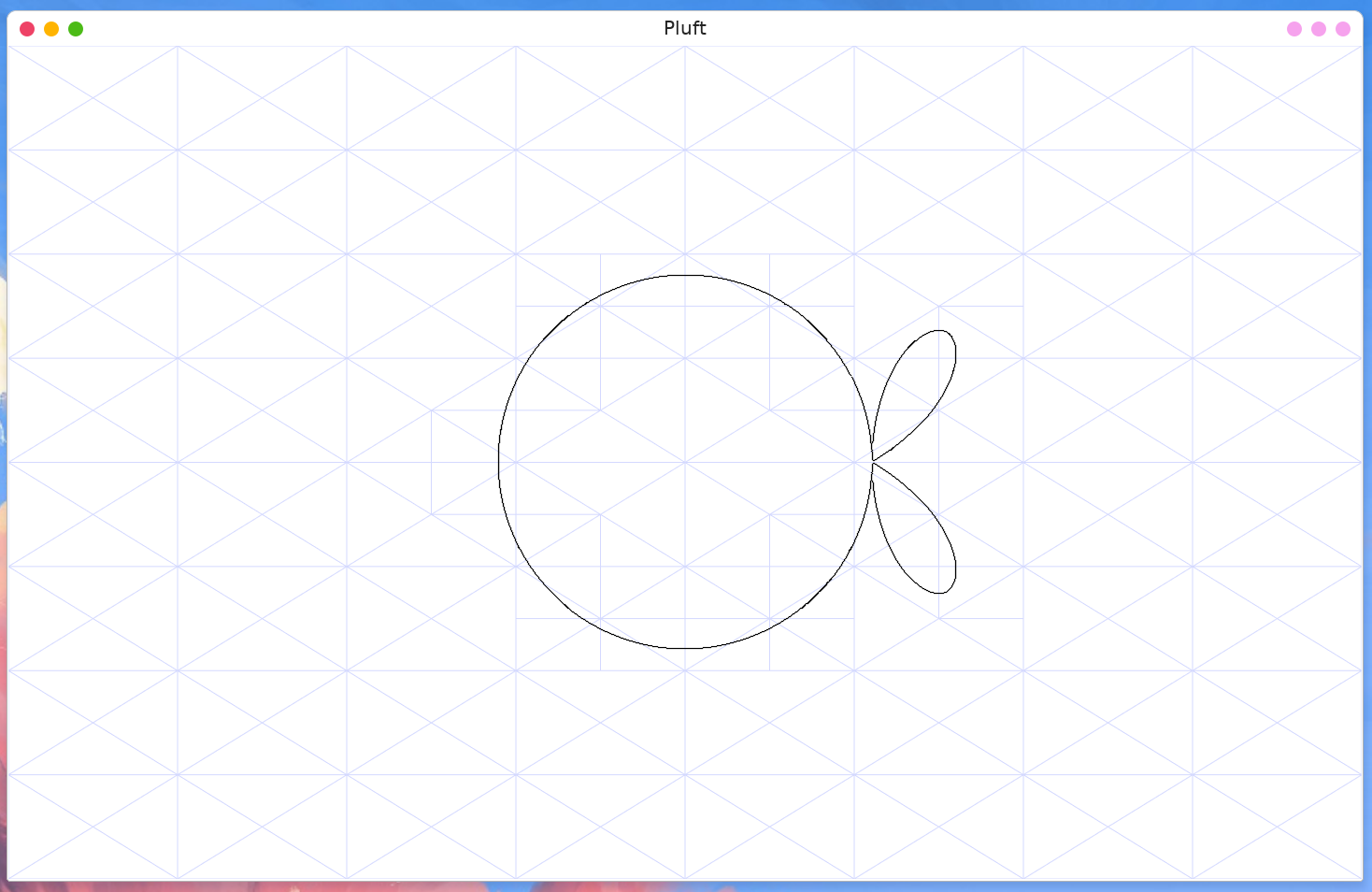
How this actually looks is as follows. The 3D curve for a circle is like this, intersecting the XY plane and forming the circle:

The regular negative gradient operation would point all the way to the bottom of the function, below zero.

But if we take the absolute value:

Now the negative gradient of every point in the surface points into the direction of the zero of the function! (except the zero itself 😁)

That is great! We just need to start at any pixel in the screen, go into that direction until we intersect the function and we have a starting pixel for the tracing algorithm.

But how do we actually compute a approximation of the gradient? 🤔

Approximating the Gradient

If we sample the differences in the function between two random points, we know that, in the direction given by those two points, the function grows or shrinks by that amount. In other words:

Given two near points p_i1, p_i2, and the function f. The function f changes by: $$\Delta_i = f(p_{i2})-f(p_{i1})$$ In the direction: $$\vec{\Delta_i} = p_{i2} - p_{i1}$$ On the vicinity of p_i1 and p_i2.

This will not, however, give us the full gradient, because not all basis vectors are represented equally when we take two points. So, we must take more samples, and the points must be chosen to lie around a circle at regular intervals (so each basis has equal representation). Then we can do:

$$\nabla f(x, y) \propto \sum_{i}{\Delta_i\vec{\Delta_i}} $$

Yay! 🦩

The simplest figure for which this can work is the regular polygon with the fewest edges: the triangle!

So, in another words, we want to create a small triangle around the point we are calculating the gradient for and sum the vectors A, B, and C times their respective Δs. The result should be proportional to the gradient, so we can normalize it to have a unit vector in the direction of the gradient:

Now we can use this to write a bit of Rust to find one point in an implicit curve, given any starting point on the plane:

fn find_pixel_on_curve(curve: Implicit, mut p: Point) -> Option<Point> {
    let mut search_distance = 20f32;
    let mut current_direction = abs_inverse_gradient(curve, p).unwrap();
    let mut previous_direction;

    for _ in 0..MAX_TRACE_SEARCH {
        // Go into the direction of -∇|f(p)|
        p = p + current_direction * search_distance;

        // We found a pixel on the curve! Early exit.
        if pixel_intersects_curve(p, curve) {
            return Some(Point::new(p.x.floor(), p.y.floor()));
        }

        previous_direction = current_direction;
        current_direction = abs_inverse_gradient(curve, p).unwrap();

        // We crossed the zero of the function, turn back moving slower
        if dot(previous_direction, current_direction) < 0.0 {
            search_distance /= 2f32;
        }
    }

    None
}

Combining

We now have a tracing algorithm that is more stable in drawing implicit curves once we have found one point in the curve. Do keep in mind that it is not perfect, it still uses the intersection function, but usually in a scale that is much more linear. It can also fail to find the starting point of the curve if there are local minima and the algorithm to find the first pixel becomes “trapped” in one of those.

To avoid that, we fist start out using the subdivision-intersection algorithm with blind search, then we refine it as usual, and then instead of simply drawing the pixels at the positions found, we TRACE the function from those points! 🤯

// Draw curve
if depth >= MAX_DEPTH {
    let triangle_center = (tri[0] + tri[1] + tri[2]) / 3.0;

    trace(
        f,
        triangle_center,
        pixels,
    );

    return;
}

Full Source Code

This article came to life from my explorations into plotting implicit functions with a little program I called Pluft.

There you can see the full working implementation of all the algorithms mentioned above and experiment with plotting different functions.

Appendix A: Interesting Figures

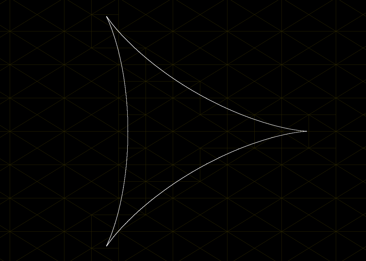
The Circle

$$z = f(x, y) = x^2+y^2-r^2$$

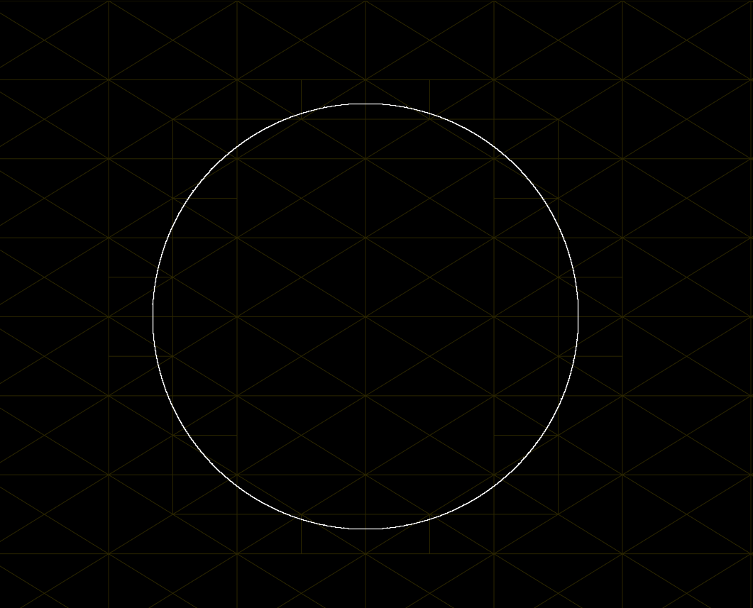
The Curved Triangle

$$z = f(x, y) = \left(x^2 + y^2 + 12ax + 9a^2\right)^2 - 4a(2x+3a)^3$$

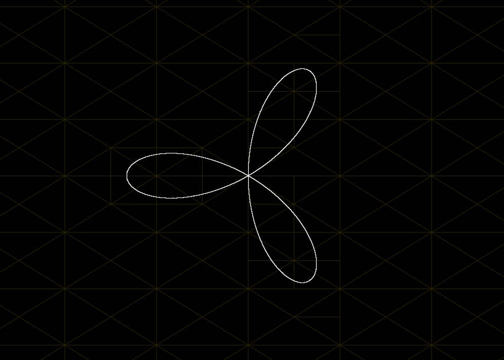
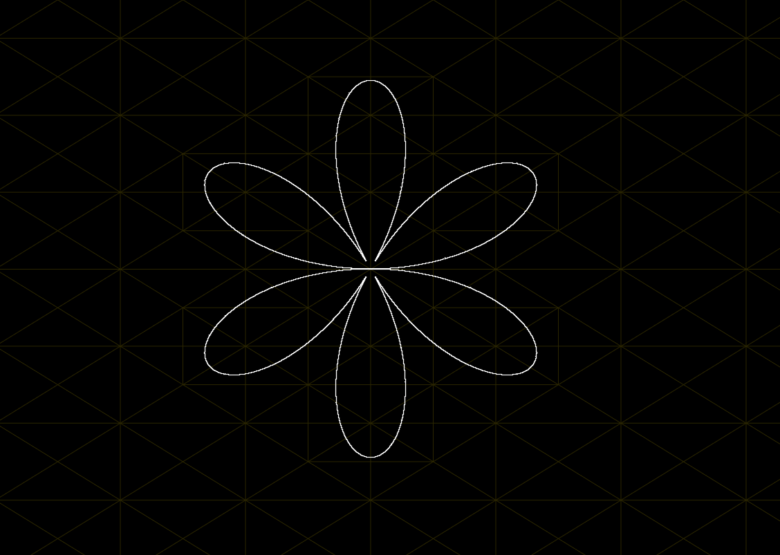
The Flower

$$z = f(x, y) = \left(3x^2-y^2\right)^2 y^2 - \left(x^2 + y^2\right)^4$$

The Knot

$$z = f(x, y) = \left(x^2 + y^2\right)\left(y^2+x\left(x+\frac{1}{2}\right)\right) - 4 \cdot \frac{1}{2} x y^2$$